Flexible and Rigid Graphs

This module implements functionality for investigating rigidity and flexibility of graphs.

The following notions from Rigidity Theory are used:

Let \(G=(V_G,E_G)\) be a graph with an edge labeling $\lambda:E_G\rightarrow \mathbb{R}_+$.

A realization $\rho:V_G\rightarrow\mathbb{R}^2$ is called compatible with $\lambda$ if $||\rho(u)-\rho(v)||=\lambda(uv)$ for all $uv\in E_G$.

The labeling $\lambda$ is called

• (proper) flexible if the number of (injective) realizations of $G$ compatible with $\lambda$ is infinite,
• rigid if the number of realizations of $G$ compatible with $\lambda$ is infinite,

where the counting is up to direct Euclidean isometries.

A graph is called movable iff it has a proper flexible labeling.

A graph is generically rigid, i.e., a generic realization defines a rigid labeling, if and only if the graph contains a Laman subgraph with the same set of vertices [Lam1970], [Pol1927].

A graph $G=(V_G,E_G)$ is called Laman if $|E_G| = 2|V_G|-3$, and $|E_H|\leq 2|V_H|-3$ for all subgraphs $H$ of $G$, see Wikipedia.

Methods

FlexRiGraph

Graph properties

is_complete()	Return if the graph is complete.
triangle_connected_components()	Return triangle connected components.

Movability

has_injective_grid_construction()	Return if there is a NAC-coloring with injective grid coordinates.
has_injective_spatial_embedding()	Return if there is a spatial embeddings for some pair of NAC-colorings.
is_movable()	Return if the graph is movable.
spatial_embeddings_four_directions()	Return injective embeddings in $\mathbb{R}^3$ with edges in 4 directions.

NAC-colorings

NAC_colorings()	Return NAC-colorings of the graph.
NAC_colorings_isomorphism_classes()	Return partition of NAC-colorings into isomorphism classes.
are_NAC_colorings_named()	Return if all NAC-colorings have a unique name.
cdc_is_complete()	Return if the constant distance closure is the complete graph.
constant_distance_closure()	Return the constant distance closure of the graph.
has_NAC_coloring()	Return if the graph has a NAC-coloring.
has_flexible_labeling()	Alias for has_NAC_coloring().
name2NAC_coloring()	Return the NAC-coloring with the given name.
set_NAC_colorings_names()	Set names of NAC-colorings according to isomorphism classes.
unicolor_pairs()	Return pairs of non-adjacent vertices linked by a unicolor path.
unicolor_path()	Return a unicolor path from u to v.

Other

graph2int()	Return the integer representation of the graph.
has_min_degree_at_least_three()	Return if all vertices have degree at least three.

Plotting

plot()

Return the plot of the graph.

print_tikz()	Print TikZ code of the graph.
show_all_NAC_colorings()	Show all NAC-colorings of the graph. The parameter ncols specifies in how many columns are the NAC colorings displayed.

Rigidity

Henneberg_sequence()	Return Henneberg sequence(s) of the graph.
Henneberg_sequence2graphs()	Return graphs of Henneberg sequence.
is_Laman()	Return whether the graph is Laman.
mixed_volume()	Return the mixed volume of the system of equations if the graph is Laman.
num_realizations()	Return the number of complex realizations if the graph is Laman.
random_realization()	Return a random realization of the graph.
realization2edge_lengths()	Return the edge lengths for realization.
realizations()	Return the realizations for given edge lengths if the graph is Laman.
system_of_equations()	Return the system of equation for edge_lengths.

Subgraphs

four_cycles()	Return all 4-cycles in the graph. INPUT:
induced_K23s()	Return all induced $K_{2,3}$ subgraphs.
triangles()	Return all triangles in the graph.

AUTHORS:

• Jan Legerský (2019-01-15): initial version
• Jan Legerský (2020-03-12): update to SageMath 9.0

TODO:

• missing documentation of methods
• missing doctests in methods
• tutorial notebooks (basics, flexibility, classification, animations…)

FlexRiGraph

class flexrilog.flexible_rigid_graph.FlexRiGraph(data, pos=None, name=None, check=True)

Bases: sage.graphs.graph.Graph

The class FlexRiGraph is inherited from sage.graphs.graph.Graph. It is a simple undirected connected graph with at least one edge. It adds functionality for rigidity and flexibility of the graph. The graph is immutable in order to prevent adding/removing edges or vertices.

INPUT:

• data: provides the information about edges. There are three possibilities:
  • FlexRiGraph(list_of_edges) – return the graph with the edges given by list_of_edges.
  • FlexRiGraph(number) – build a graph whose adjacence matrix is given as follows: the binary expansion of the integer number is written row by row into the upper triangle, excluding the diagonal, and symmetrically also into the lower triangle.
  • FlexRiGraph(graph) – return the graph with the same edges, positions and name as graph.
• name – gives the graph a name
• pos – a positioning dictionary. For example, to draw 4 vertices on a square pos={0: [-1,-1], 1: [ 1,-1], 2: [ 1, 1], 3: [-1, 1]}.
• check (boolean) – If True (default), then it is checked whether the graph connected and has at least one edge.

EXAMPLES:

The single edge graph:

sage: from flexrilog import FlexRiGraph
sage: G = FlexRiGraph(1); G
FlexRiGraph with the vertices [0, 1] and edges [(0, 1)]

Graphs without edges are not allowed:

sage: G = FlexRiGraph([]); G
Traceback (most recent call last):
...
ValueError: The graph must have at least one edge.

A named graph given by integer representation with specified positions:

sage: G = FlexRiGraph(7916, name='3-prism',
....:       pos={0: [0.6, 0.4], 1: [0, 1.4], 2: [1, 1.4],
....:            3: [1, 0], 4: [0, 0], 5: [0.6, 1]}); G
3-prism: FlexRiGraph with the vertices [0, 1, 2, 3, 4, 5] and edges [(0, 3), (0, 4), (0, 5), (1, 2), (1, 4), (1, 5), (2, 3), (2, 5), (3, 4)]
sage: from flexrilog import GraphGenerator
sage: G == GraphGenerator.ThreePrismGraph()
True

The dictionary pos is used when plotting: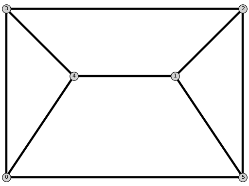

The 3-cycle graph given by the list of edges:

sage: G = FlexRiGraph([[0,1],[1,2],[0,2]], name='3-cycle'); G
3-cycle: FlexRiGraph with the vertices [0, 1, 2] and edges [(0, 1), (0, 2), (1, 2)]

An instance of sage.graphs.graph.Graph can be used:

sage: L = FlexRiGraph(graphs.CompleteBipartiteGraph(2,3)); L
Complete bipartite graph of order 2+3: FlexRiGraph with the vertices [0, 1, 2, 3, 4] and edges [(0, 2), (0, 3), (0, 4), (1, 2), (1, 3), (1, 4)]

TODO:

Other inputs: adjacency matrix

Henneberg_sequence(onlyOne=True)

Return Henneberg sequence(s) of the graph.

The graph is Laman if and only if it can be constructed using Henneberg steps, see Wikipedia.

INPUT:

• onlyOne – if True (default), then only one Henneberg sequence is returned (if exists). Otherwise, all sequences are found.

OUTPUT:

The sequence is reversed - it describes the order of removing vertices by undoing Henneberg steps : ('I',u) denotes that the vertex u of degree two is removed and ('II', u, (v, w)) means that the vertex u of degree three is removed and the edge [v, w] is added. If there is no Henneberg sequence, then the output is None.

EXAMPLES:

A Henneberg sequence for 3-prism:

sage: from flexrilog import FlexRiGraph
sage: G = FlexRiGraph(7916); G
FlexRiGraph with the vertices [0, 1, 2, 3, 4, 5] and edges [(0, 3), (0, 4), (0, 5), (1, 2), (1, 4), (1, 5), (2, 3), (2, 5), (3, 4)]
sage: print(G.Henneberg_sequence())
[('II', 0, (3, 5)), ('I', 4), ('I', 1), ('I', 2)]

4-cycle is not Laman:

sage: G = FlexRiGraph([[0,1],[1,2],[2,3],[0,3]])
sage: G.Henneberg_sequence()==None
True

The complete graph $K_4$ is not Laman:

sage: G = FlexRiGraph([(0, 1), (0, 2), (0, 3), (1, 2), (1, 3), (2, 3)])
sage: G.Henneberg_sequence()==None
True

All Henneberg sequence of $K_4$ with one edge removed:

sage: G = FlexRiGraph([[0,1],[1,2],[2,3],[0,3],[0,2]])
sage: G.Henneberg_sequence()
[('I', 1), ('I', 0)]
sage: G.Henneberg_sequence(onlyOne=False)
[[('I', 1), ('I', 0)],
[('I', 1), ('I', 0)],
[('I', 1), ('I', 0)],
[('I', 1), ('I', 0)],
[('I', 1), ('I', 0)],
[('I', 1), ('I', 0)],
[('II', 0, (1, 3)), ('I', 1)],
[('II', 0, (1, 3)), ('I', 1)],
[('II', 0, (1, 3)), ('I', 1)],
[('II', 2, (3, 1)), ('I', 0)],
[('II', 2, (3, 1)), ('I', 0)],
[('II', 2, (3, 1)), ('I', 0)]]

Henneberg_sequence2graphs(seq)

Return graphs of Henneberg sequence.

INPUT:

• seq - sequence of Henneberg steps as outputted by Henneberg_sequence().

OUTPUT:

Graphs obtained by applying the Henneberg sequence seq.

EXAMPLE:

sage: from flexrilog import GraphGenerator
sage: G = GraphGenerator.ThreePrismGraph()
sage: seq = G.Henneberg_sequence(); seq
[('II', 0, (3, 5)), ('I', 4), ('I', 1), ('I', 2)]
sage: G.Henneberg_sequence2graphs(seq)
[3-prism: Graph on 2 vertices,
3-prism: Graph on 3 vertices,
3-prism: Graph on 4 vertices,
3-prism: Graph on 5 vertices,
3-prism: Graph on 6 vertices]

NAC_colorings()

Return NAC-colorings of the graph.

If the NAC-colorings are already stored, then they are just returned, otherwise computed.

OUTPUT:

Only one NAC-coloring per conjugacy class is return.

EXAMPLES:

sage: from flexrilog import GraphGenerator
sage: G = GraphGenerator.ThreePrismGraph()
sage: G.NAC_colorings()
[NAC-coloring with red edges [[0, 3], [0, 4], [1, 2], [1, 5], [2, 5], [3, 4]] and blue edges [[0, 5], [1, 4], [2, 3]]]

sage: from flexrilog import FlexRiGraph
sage: K = FlexRiGraph(graphs.CompleteGraph(4))
sage: K.NAC_colorings()
[]

sage: K = FlexRiGraph(graphs.CompleteBipartiteGraph(3,3))
sage: len(K.NAC_colorings())
15

The NAC-colorings are cached:

sage: K = FlexRiGraph(graphs.CompleteBipartiteGraph(3,3))
sage: %time len(K.NAC_colorings()) # doctest: +SKIP
CPU times: user 418 ms, sys: 22.4 ms, total: 440 ms
Wall time: 411 ms
15
sage: %time len(K.NAC_colorings()) # doctest: +SKIP
CPU times: user 36 µs, sys: 3 µs, total: 39 µs
Wall time: 55.1 µs
15

TODO:

Implement as an iterator?

NAC_colorings_isomorphism_classes()

Return partition of NAC-colorings into isomorphism classes.

See flexrilog.NAC_coloring.NACcoloring.is_isomorphic() for the definition of two NAC-colorings being isomorphic.

EXAMPLE:

sage: from flexrilog import FlexRiGraph
sage: G = FlexRiGraph(graphs.CompleteBipartiteGraph(2,3))
sage: isomorphism_classes = G.NAC_colorings_isomorphism_classes()
sage: len(isomorphism_classes)
3
sage: [len(cls) for cls in isomorphism_classes]
[1, 3, 3]
sage: for cls in isomorphism_classes: print(cls[0])
NAC-coloring with red edges [[0, 2], [0, 3], [0, 4]] and blue edges [[1, 2], [1, 3], [1, 4]]
NAC-coloring with red edges [[0, 2], [0, 3], [1, 2], [1, 3]] and blue edges [[0, 4], [1, 4]]
NAC-coloring with red edges [[0, 2], [0, 3], [1, 4]] and blue edges [[0, 4], [1, 2], [1, 3]]

are_NAC_colorings_named()

Return if all NAC-colorings have a unique name.

cdc_is_complete(active_colorings=None)

Return if the constant distance closure is the complete graph.

Theorem [GLS2018a]

A graph $G$ is movable if and only the constant distance closure of $G$ is movable.

Corollary

If $G$ is movable, then the constant distance closure of $G$ is not complete.

EXAMPLES:

sage: from flexrilog import GraphGenerator
sage: G = GraphGenerator.ThreePrismGraph()
sage: G.cdc_is_complete()
False

sage: G = GraphGenerator.SmallestFlexibleLamanGraph()
sage: G.cdc_is_complete()
True

sage: G = GraphGenerator.MaxEmbeddingsLamanGraph(7)
sage: G.cdc_is_complete()
True

constant_distance_closure(active_colorings=None, save_colorings=False)

Return the constant distance closure of the graph.

Let $\operatorname{U}(G)$ denote the set of all pairs $\{u,v\}\subset V_G$ such that $uv\notin E_G$ and there exists a path from $u$ to $v$ which is unicolor for all NAC-colorings $\delta$ of $G$. If there exists a sequence of graphs $G=G_0, \dots, G_n$ such that $G_i=(V_{G_{i-1}},E_{G_{i-1}} \cup \operatorname{U}(G_{i-1}))$ for $i\in\{1,\dots,n\}$ and $\operatorname{U}(G_n)=\emptyset$, then the graph $G_n$ is called the constant distance closure of $G$.

INPUT:

• active_colorings (default None) – if specified, then they are used instead of all NAC-colorings of the graph.
• save_colorings (default False) – if True, then the constant distance closure is returned with the NAC-colorings obtained during the computation.

EXAMPLES:

sage: from flexrilog import GraphGenerator
sage: G = GraphGenerator.ThreePrismGraph()
sage: CDC = G.constant_distance_closure()
sage: CDC.is_isomorphic(G)
True

sage: G = GraphGenerator.SmallestFlexibleLamanGraph()
sage: CDC = G.constant_distance_closure()
sage: CDC.is_isomorphic(graphs.CompleteGraph(5))
True

sage: from flexrilog import FlexRiGraph
sage: G = FlexRiGraph(1256267)
sage: CDC = G.constant_distance_closure()
sage: len(CDC.edges())-len(G.edges())
1

TODO:

An interesting example with less NAC-colorings.

Speed up using triangle-components?

four_cycles(only_with_NAC=False)

Return all 4-cycles in the graph.

INPUT:

• only_with_NAC (default False) – if True, then a 4-cycle is in the returned list only if there exists a NAC-coloring of the graph which is not unicolor on the 4-cycle.

OUTPUT:

List of all (in terms of the vertex set) 4-cycles given by ordered tuples of their vertices.

EXAMPLES:

sage: from flexrilog import GraphGenerator
sage: G = GraphGenerator.ThreePrismGraph()
sage: G.four_cycles()
[(0, 3, 2, 5), (0, 4, 1, 5), (1, 2, 3, 4)]

sage: from flexrilog import FlexRiGraph
sage: len(FlexRiGraph(graphs.CompleteGraph(7)).four_cycles()) == binomial(7,4)*3
True

sage: FlexRiGraph(graphs.CycleGraph(7)).four_cycles()
[]

graph2int(canonical=True)

Return the integer representation of the graph.

The graph has integer representation N if the binary expansion of N equals the sequence obtained by concatenation of the rows of the upper triangle of the adjacency matrix, excluding the diagonal.

INPUT:

• canonical (boolean) – if True (default), then the adjacency matrix of the isomorphic graph obtained by canonical_label() is used. In this case, the isomorphic graphs have the same integer representation.

EXAMPLES:

sage: from flexrilog import FlexRiGraph
sage: G = FlexRiGraph(graphs.CycleGraph(4)); G
Cycle graph: FlexRiGraph with the vertices [0, 1, 2, 3] and edges [(0, 1), (0, 3), (1, 2), (2, 3)]
sage: G.graph2int(canonical=False)
45
sage: G.adjacency_matrix()
[0 1 0 1]
[1 0 1 0]
[0 1 0 1]
[1 0 1 0]
sage: int('101101',2)
45
sage: G.graph2int()
30
sage: H = FlexRiGraph(30); H
FlexRiGraph with the vertices [0, 1, 2, 3] and edges [(0, 2), (0, 3), (1, 2), (1, 3)]
sage: H.graph2int()
30

has_NAC_coloring(certificate=False)

Return if the graph has a NAC-coloring.

INPUT:

• certificate (boolean) – if False (default), then only boolean value is returned. Otherwise, the output is (True, NACcoloring) or (False, None).

EXAMPLES:

sage: from flexrilog import GraphGenerator
sage: G = GraphGenerator.ThreePrismGraph()
sage: G.has_NAC_coloring()
True
sage: G.has_NAC_coloring(certificate=True)
(True, NAC-coloring with red edges [[0, 3], [0, 4], [1, 2], [1, 5], [2, 5], [3, 4]] and blue edges [[0, 5], [1, 4], [2, 3]])

sage: from flexrilog import FlexRiGraph
sage: K = FlexRiGraph(graphs.CompleteGraph(4))
sage: K.has_NAC_coloring()
False
sage: K.has_NAC_coloring(certificate=True)
(False, None)

sage: K = FlexRiGraph(graphs.CompleteBipartiteGraph(3,3))
sage: K.has_NAC_coloring(certificate=True)
(True, NAC-coloring with red edges [[0, 3], [0, 4], [0, 5], [1, 3], [1, 4], [1, 5]] and blue edges [[2, 3], [2, 4], [2, 5]])

has_flexible_labeling(certificate=False)

Alias for has_NAC_coloring().

A flexible labeling exists if and only if a NAC-coloring exists (Theorem 3.1 in [GLS2018]).

has_injective_grid_construction(certificate=False)

Return if there is a NAC-coloring with injective grid coordinates.

See flexrilog.NAC_coloring.NACcoloring.grid_coordinates().

INPUT:

• certificate (boolean) – if False (default), then only boolean value is returned. Otherwise, the output is (True, delta) or (False, None), where the delta is a NAC-coloring giving injective grid construction.

EXAMPLES:

sage: from flexrilog import GraphGenerator
sage: G = GraphGenerator.ThreePrismGraph()
sage: G.has_injective_grid_construction(certificate=True)
(True, NAC-coloring with red edges [[0, 3], [0, 4], [1, 2], [1, 5], [2, 5], [3, 4]] and blue edges [[0, 5], [1, 4], [2, 3]])

sage: from flexrilog import GraphGenerator
sage: G = GraphGenerator.SmallestFlexibleLamanGraph()
sage: G.has_injective_grid_construction()
False

has_injective_spatial_embedding(certificate=False, onlyOne=True)

Return if there is a spatial embeddings for some pair of NAC-colorings.

The method runs spatial_embeddings_four_directions() for all pairs of NAC-colorings of the graph.

INPUT:

• certificate – if False (default), then only boolean is returned. Otherwise, the output contains also the pair of NAC-colorings giving an injective spatial embedding (if it exists, otherwise None).
• onlyOne – if True, then only one pair on NAC-colorings is returned as a certificate, otherwise a list of all posibble ones.

EXAMPLES:

sage: from flexrilog import GraphGenerator
sage: G = GraphGenerator.ThreePrismGraph()
sage: G.has_injective_spatial_embedding(certificate=True)
(False, None)

sage: G = GraphGenerator.Q1Graph()
sage: G.has_injective_spatial_embedding(certificate=True)
(True, [eta: NAC-coloring with 7 red edges and 4 blue edges , epsilon24: NAC-coloring with 7 red edges and 4 blue edges ])

sage: G.has_injective_spatial_embedding(certificate=True, onlyOne=False) # long time
(True,
[[eta: NAC-coloring with 7 red edges and 4 blue edges ,
...
epsilon14: NAC-coloring with 7 red edges and 4 blue edges ]])

has_min_degree_at_least_three()

Return if all vertices have degree at least three.

induced_K23s()

Return all induced $K_{2,3}$ subgraphs.

OUTPUT:

List of all induced $K_{2,3}$ subgraphs given by of their vertices.

EXAMPLES:

sage: from flexrilog import GraphGenerator
sage: G = GraphGenerator.Q1Graph()
sage: G.induced_K23s()
[[1, 2, 7, 3, 4], [3, 4, 5, 1, 7], [3, 4, 6, 2, 7]]

sage: from flexrilog import FlexRiGraph
sage: FlexRiGraph(graphs.CompleteGraph(7)).induced_K23s()
[]

sage: len(FlexRiGraph(graphs.CompleteBipartiteGraph(4,6)).induced_K23s()) == binomial(4,3)*binomial(6,2) + binomial(4,2)*binomial(6,3)
True

is_Laman(algorithm=None, certificate=False)

Return whether the graph is Laman.

A graph $G=(V_G,E_G)$ is called Laman if $|E_G| = 2|V_G|-3$, and $|E_H|\leq 2|V_H|-3$ for all subgraphs $H$ of $G$, see Wikipedia.

INPUT:

• algorithm (string) – there are two options:
  • If algorithm = "definition", then the Laman condition on subgraphs is checked naively (VERY SLOW!!).
  • If algorithm = "Henneberg" (default), then a sequence of Henneberg steps is attempted to be found (SLOW!!).
• certificate (boolean) – If certificate = False (default), then the returns only boolean. Otherwise:
  • If algorithm = "Henneberg", then it either answers (True, s) when the graph is Laman and can be constructed by Henneberg sequence s, or (False, None) when it is not Laman. See Henneberg_sequence().
  • If algorithm = "definition", then the certificate is None if the graph is Laman, otherwise (False, H), where H is the graph that violates the condition.

EXAMPLES:

3-prism is Laman:

sage: from flexrilog import GraphGenerator
sage: G = GraphGenerator.ThreePrismGraph()
sage: G.is_Laman()
True
sage: G.is_Laman(certificate=True)
(True, [('II', 0, (3, 5)), ('I', 4), ('I', 1), ('I', 2)])
sage: G.is_Laman(algorithm='definition')
True

4-cycle is not Laman:

sage: from flexrilog import FlexRiGraph
sage: G = FlexRiGraph([[0,1],[1,2],[2,3],[0,3]])
sage: G.is_Laman(algorithm='definition', certificate=True)
(False, Graph on 4 vertices)
sage: G.is_Laman(algorithm='Henneberg', certificate=True)
(False, None)

The complete graph $K_4$ is not Laman:

sage: G = FlexRiGraph([(0, 1), (0, 2), (0, 3), (1, 2), (1, 3), (2, 3)])
sage: G.is_Laman(algorithm='definition', certificate=True)
(False, Graph on 4 vertices)
sage: G.is_Laman(algorithm='Henneberg', certificate=True)
(False, None)

TODO:

Implementation of pebble game algorithm.

is_complete()

Return if the graph is complete.

is_movable()

Return if the graph is movable.

The method tests the necessary condition cdc_is_complete() and sufficient ones: has_injective_grid_construction(), has_injective_spatial_embedding() and is_bipartite().

OUTPUT:

• If the graph has no NAC-coloring, then ('no', 'no NAC-coloring') is returned.
• If the constant distance closure is the complete graph, then ('no', 'CDC is complete') is returned.
• If the graph is bipartite, then ('yes', 'bipartite')
• If the graph has a NAC-coloring giving an injective grid construction, then ('yes', 'grid construction').
• If the graph has a pair of NAC-coloring giving an injective spatial embedding, then ('yes', 'spatial embedding').
• Otherwise, ('cannot decide','').

EXAMPLES:

sage: from flexrilog import GraphGenerator
sage: GraphGenerator.LamanGraphs(4)[0].is_movable()
('no', 'no NAC-coloring')

sage: from flexrilog import GraphGenerator
sage: GraphGenerator.MaxEmbeddingsLamanGraph(7).is_movable()
('no', 'CDC is complete')

sage: from flexrilog import FlexRiGraph
sage: FlexRiGraph(graphs.CompleteBipartiteGraph(3,3)).is_movable()
('yes', 'bipartite')

sage: GraphGenerator.ThreePrismGraph().is_movable()
('yes', 'grid construction')

sage: GraphGenerator.Q1Graph().is_movable() # long time
('yes', 'spatial embedding')

sage: GraphGenerator.S1Graph().is_movable() # long time
('cannot decide', '')

sage: len([G for G in GraphGenerator.LamanGraphs(6) if G.is_movable()[0]=='yes'])
2

TODO:

Graphs with a generic flexible labeling (not spanned by a Laman graph).

mixed_volume(fixed_edge=None, check=True, full_list=False)

Return the mixed volume of the system of equations if the graph is Laman.

The method uses phcpy to compute the mixed volume of the system of equations (phcpy must be installed) This gives an upper bound on the number of realizations.

INPUT:

• fixed_edge - the system of equations is constructed with this fixed edge. If None (default), then the minimum mixed volume over all edges is returned.
• check - if True (default), then it is checked that the graph is Laman.
• full_list (default False) - if True and fixed_edge==None, then the list of pairs [edge, MV] is returned.

EXAMPLES:

sage: import phcpy # random, optional - phcpy
sage: # the previous import is just because of the message that phcpy prints when imported
sage: from flexrilog import GraphGenerator
sage: GraphGenerator.ThreePrismGraph().mixed_volume() # optional - phcpy
32

sage: GraphGenerator.MaxEmbeddingsLamanGraph(7).mixed_volume() # optional - phcpy
64
sage: GraphGenerator.MaxEmbeddingsLamanGraph(7).mixed_volume([1,5]) # optional - phcpy
96
sage: GraphGenerator.MaxEmbeddingsLamanGraph(7).mixed_volume(full_list=True) # optional - phcpy
[[(1, 2), 128],
...
[(6, 7), 64]]

name2NAC_coloring(name)

Return the NAC-coloring with the given name.

TODO:

Implement using a dictionary instead of traversing the whole list each time.

num_realizations(check=True)

Return the number of complex realizations if the graph is Laman.

The method uses the package lnumber by J. Capco, see also [CGGKLS2018a].

EXAMPLE:

sage: from flexrilog import GraphGenerator
sage: [GraphGenerator.MaxEmbeddingsLamanGraph(i).num_realizations() for i in range(6,13)] # optional - lnumber
[24, 56, 136, 344, 880, 2288, 6180]

plot(NAC_coloring=None, show_triangle_components=False, name_in_title=True, **kwargs)

Return the plot of the graph.

INPUT:

• NAC_coloring – if an instance of NACcoloring is provided, then the edges are colored accordingly.
• show_triangle_components (default False) – if True, then the edges in the same $\triangle$-component have the same color.
• for other options, see sage.graphs.generic_graph.GenericGraph.plot(). For instance, pos specifies the positions of the vertices.

EXAMPLES:

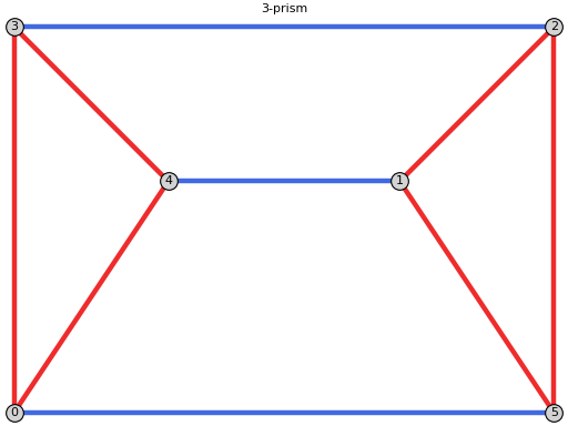
sage: from flexrilog import GraphGenerator
sage: G = GraphGenerator.ThreePrismGraph()
sage: print(G.plot(NAC_coloring=G.NAC_colorings()[0]))
Graphics object consisting of 16 graphics primitives

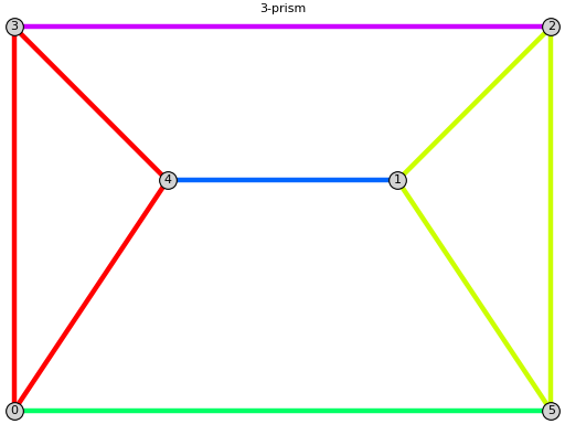
sage: G.triangle_connected_components()
[[[0, 3], [0, 4], [3, 4]], [[1, 2], [1, 5], [2, 5]], [[0, 5]], [[1, 4]], [[2, 3]]]
sage: print(G.plot(show_triangle_components=True))
Graphics object consisting of 16 graphics primitives

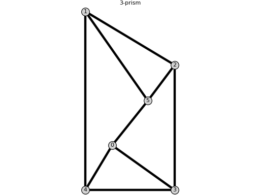
sage: print(G.plot(pos={0: [0.3, 0.5], 1: [0, 2], 2: [1, 1.4], 3: [1, 0], 4: [0, 0], 5: [0.7, 1]}))
Graphics object consisting of 16 graphics primitives

print_tikz(colored_edges=[], color_names=['edge'], vertex_style='vertex', scale=1)

Print TikZ code of the graph.

random_realization()

Return a random realization of the graph.

EXAMPLE:

sage: from flexrilog import GraphGenerator
sage: GraphGenerator.ThreePrismGraph().random_realization() # random
{0: (1.2663140331566647, 6.798542831673373),
...
5: (1.938458777654558, 4.519218477998938)}

realization2edge_lengths(realization)

Return the edge lengths for realization.

EXAMPLE:

sage: from flexrilog import GraphGenerator
sage: G = GraphGenerator.ThreePrismGraph()
sage: G.realization2edge_lengths(G.random_realization()) # random
{(0, 3): 0.5656854249492381,
...
(3, 4): 1}

realizations(edge_lengths, fixed_edge=None, check=True, tolerance_real=1e-08, prec='d', num_tasks=2)

Return the realizations for given edge lengths if the graph is Laman.

The method uses phcpy to compute the solutions of the system of equations (phcpy must be installed)

INPUT:

• edge_lengths – a dictionary assigning a length to each edge.
• fixed_edge (default None) – if specified, then it is used as the fixed edge. Otherwise, one of the edges giving the minimal mixed volume is used
• tolerance_real (default 1e-8) – a solution is considered real if the absolute value of the imaginary part of each coordinate is smaller than this number.
• prec (default 'd') – precision used in phcpy: 'd' for double precision, 'dd' for double double preicsion (about 32 decimal places) and 'qd' for quad double precision (about 64 decimal places).
• num_tasks – number of threads used.

OUTPUT:

A pair [result_real, result_complex] of two lists is returned. The first list contains dictionaries with real realizations, whereas the second one with the complex solutions. If the fixed_edge is in a 3-cycle, then realizations only with one orienation of the triangle are returned.

EXAMPLE:

sage: import phcpy # random, optional - phcpy
sage: # the previous import is just because of the message that phcpy prints when imported
sage: from flexrilog import GraphGenerator
sage: L = {(1, 2): 3, (1, 5): 4, (0, 5): 5, (0, 4): 3, (2, 3): 5, (0, 3): 2, (3, 4): 4, (2, 5): 2, (1, 4): 5}
sage: res_RR, res_CC = GraphGenerator.ThreePrismGraph().realizations(L,[4,3]); (len(res_RR), len(res_CC)) # optional - phcpy
(10, 2)
sage: res_RR # random, optional - phcpy
[{0: (2.62500000000000, 1.45236875482778),
1: (-0.988599837464227, 4.90129272349303),
2: (1.99414754086938, 4.58001702095087),
3: (4, 0),
4: (0, 0),
5: (2.6986546781728, 6.45182622423216)},
...
5: (7.47928649393724, 2.65066030314919)}]

Some of the realizations from the example above:

set_NAC_colorings_names(cls_names=[])

Set names of NAC-colorings according to isomorphism classes.

The NAC-colorings in the same class have the same name with a different index.

INPUT:

• cls_names (default [])– if specified, then these names are taken for the isomorphism classes. Otherwise, Greek letters are taken.

EXAMPLE:

sage: from flexrilog import FlexRiGraph
sage: G = FlexRiGraph(graphs.CompleteBipartiteGraph(2,3))
sage: G.set_NAC_colorings_names()
sage: G.NAC_colorings()
[alpha: NAC-coloring with red edges [[0, 2], [0, 3], [0, 4]] and blue edges [[1, 2], [1, 3], [1, 4]],
beta1: NAC-coloring with red edges [[0, 2], [0, 3], [1, 2], [1, 3]] and blue edges [[0, 4], [1, 4]],
gamma1: NAC-coloring with red edges [[0, 2], [0, 3], [1, 4]] and blue edges [[0, 4], [1, 2], [1, 3]],
beta2: NAC-coloring with red edges [[0, 2], [0, 4], [1, 2], [1, 4]] and blue edges [[0, 3], [1, 3]],
gamma2: NAC-coloring with red edges [[0, 2], [0, 4], [1, 3]] and blue edges [[0, 3], [1, 2], [1, 4]],
beta3: NAC-coloring with red edges [[0, 2], [1, 2]] and blue edges [[0, 3], [0, 4], [1, 3], [1, 4]],
gamma3: NAC-coloring with red edges [[0, 2], [1, 3], [1, 4]] and blue edges [[0, 3], [0, 4], [1, 2]]]

show_all_NAC_colorings(ncols=3, only_return=False)

Show all NAC-colorings of the graph.

The parameter ncols specifies in how many columns are the NAC colorings displayed.

spatial_embeddings_four_directions(delta_1, delta_2, vertex_at_origin=None)

Return injective embeddings in $\mathbb{R}^3$ with edges in 4 directions.

The method attempts to embedd injectively the vertices of the graph into $\mathbb{R}^3$ so that two edges are parallel if and only if they obtain the same colors by delta_1 and delta_2. The four possible directions are (1,0,0), (0,1,0), (0,0,1) and (-1,-1,-1). If such an embedding exists, then the graph is movable:

Lemma [GLS2018a]

Let $G=(V,E)$ be a graph with an injective embedding $\omega:V\rightarrow\mathbb{R}^3$ such that for every edge $uvin E$, the vector $\omega(u)-\omega(v)$ is parallel to one of the four vectors $(1,0,0)$, $(0,1,0)$, $(0,0,1)$, $(-1,-1,-1)$, and all four directions are present. Then $G$ is movable.

Moreover, there exist two NAC-colorings such that two edges are parallel in the embedding $\omega$ if and only if they receive the same pair of colors.

INPUT:

• delta_1 and delta_2 – NAC-colorings
• vertex_at_origin – if None (default), then the first vertex is placed to the origin.

OUTPUT:

A dictionary with parametrized positions of vertices, if the embedding exists, otherwise None.

EXAMPLE:

sage: from flexrilog import GraphGenerator
sage: G = GraphGenerator.Q1Graph()
sage: G.spatial_embeddings_four_directions(G.name2NAC_coloring('epsilon13'), G.name2NAC_coloring('epsilon24'))
{1: (0, 0, 0),
 2: (2*a, a, a),
 3: (a, a, a),
 4: (a, 0, 0),
 5: (0, -a, 0),
 6: (2*a, a, 2*a),
 7: (a, 0, a)}

system_of_equations(edge_lengths, fixed_edge)

Return the system of equation for edge_lengths.

The method returns the system of equations for edge lengths with new variables for the squares of distances of vertices from the origin in order to decrease the mixed volume of the system.

INPUT:

• edge_lengths – a dictionary assigning every edge a length.
• fixed_edge – the first vertex is placed to the origin whereas the second one on the x-axis.

OUTPUT:

A pair [eqs, v] is returned, where eqs` are the equations and ``v is a vertex adjacent to both vertices of fixed_edge if it exists, or None otherwise. If it exists, then the triangle is fixed instead of just the edge, in order to simplify the system.

EXAMPLES:

sage: from flexrilog import GraphGenerator
sage: G = GraphGenerator.ThreePrismGraph()
sage: L = {(0, 3): 2, (0, 4): 3, (0, 5): 5, (1, 2): 3, (1, 4): 5, (1, 5): 4, (2, 3): 5, (2, 5): 2, (3, 4): 4 }
sage: G.system_of_equations(L, [4,3])  # random
[[s5 - 5.25000000000000*x5 - 2.90473750965556*y5 - 16.0000000000000,
...
-x2^2 - y2^2 + s2, -x5^2 - y5^2 + s5], 0]

triangle_connected_components()

Return triangle connected components.

Two edges are in relation if they are in the same 3-cycle subgraph. The equivalence classes of the reflexive-transitive closure of this relation are called $\triangle$-connected components [GLS2018].

OUTPUT:

Partition of the edges into the $\triangle$-connected components.

EXAMPLE:

sage: from flexrilog import FlexRiGraph
sage: G = FlexRiGraph([(1,6),(2,6),(0,6),(0, 3), (0, 4),
....: (0, 5), (1, 2), (1, 4), (1, 5), (2, 3), (2, 5), (3, 4)]); G
FlexRiGraph with 7 vertices and 12 edges
sage: G.triangle_connected_components()
[[[0, 3], [0, 4], [3, 4]], [[1, 2], [1, 5], [1, 6], [2, 5], [2, 6]], [[0, 5]], [[0, 6]], [[1, 4]], [[2, 3]]]

sage: from flexrilog import GraphGenerator
sage: G = GraphGenerator.ThreePrismGraph()
sage: G.triangle_connected_components()
[[[0, 3], [0, 4], [3, 4]], [[1, 2], [1, 5], [2, 5]], [[0, 5]], [[1, 4]], [[2, 3]]]

TODO:

Change so that the edge labels are not used (without creating extra copy).

triangles()

Return all triangles in the graph.

OUTPUT:

List of all triangles given by their vertices.

EXAMPLES:

Bipartite graphs have no triangles:

sage: from flexrilog import FlexRiGraph
sage: G = FlexRiGraph(graphs.CompleteBipartiteGraph(2,3))
sage: G.triangles()
[]

The 3-prism graph has two triangles:

sage: from flexrilog import GraphGenerator
sage: G = GraphGenerator.ThreePrismGraph()
sage: G.triangles()
[[0, 3, 4], [1, 2, 5]]

The complete graph on 5 vertices:

sage: len(FlexRiGraph(graphs.CompleteGraph(5)).triangles()) == binomial(5,3)
True

unicolor_pairs(active_colorings)

Return pairs of non-adjacent vertices linked by a unicolor path.

INPUT:

• active_colorings – colorings considered for unicolor paths.

OUTPUT:

List of pairs of non-adjacent vertices u and v connected by a unicolor path path in the form [[u,v],path].

unicolor_path(u, v, active_colorings=None)

Return a unicolor path from u to v.

A path is unicolor if for all NAC-colorings $\delta$ of the graph, $|\{\delta(e):e\in E_G\}|=1$.

INPUT:

• u and v – start and endpoint.
• active_colorings (default None) – if specified, then only the given colorings are considered instead of all.

OUTPUT:

A path given by vertices or [] if there is none.

EXAMPLES:

sage: from flexrilog import GraphGenerator
sage: G = GraphGenerator.SmallestFlexibleLamanGraph()
sage: G.unicolor_path(2,3)
[2, 0, 1, 3]

sage: G = GraphGenerator.ThreePrismGraph()
sage: G.unicolor_path(2,3)
[2, 3]
sage: G.has_edge(2,3)
True
sage: G.unicolor_path(1,3)
[]

sage: G = GraphGenerator.MaxEmbeddingsLamanGraph(8)
sage: G.unicolor_path(2,4)
[]
sage: G.unicolor_path(2,4, active_colorings=G.NAC_colorings()[-2:])
[2, 1, 4]